생각하는 기계?
뇌를 모방한 알고리즘을 만들 수 없을까? 뉴런은 어떻게 동작을 할까?…
이런 고민에서 다음과 같은 이론이 생겨난다.
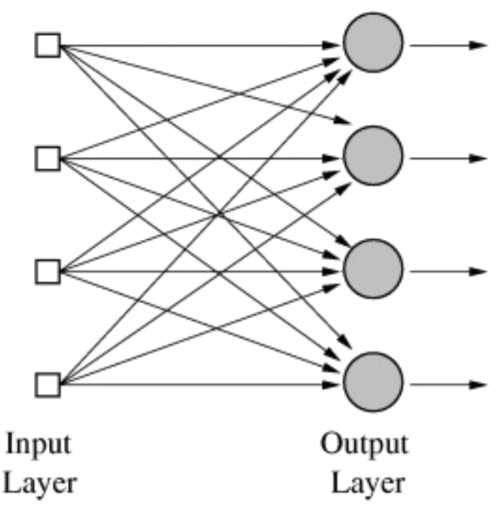
x라는 신호가 들어오면 w(weight)라는 값으로 곱해지고 이러한 신호를 모두 더한 후 편향(bias)값을 더한 다음, ‘활성화 함수(activation function)’를 통해 계산된 값에 대해 0과 1로 출력하도록 뉴런을 구현하면 어떨까?
예를 들어서 기존에 있던 로지스틱 회귀의 가설을:
\(H(X) = \frac{1}{1+e^{-W^TX}}\)
\(H(X) = \frac{1}{1+e^{-W^TX}}\)
\(H(X) = \frac{1}{1+e^{-W^TX}}\)
이런 식으로 반복한다면 어떨까.
AND OR 문제
AND
0 + 0 = 0
0 + 1 = 0
1 + 0 = 0
1 + 1 = 1
OR
0 + 0 = 0
0 + 1 = 1
1 + 0 = 1
1 + 1 = 1
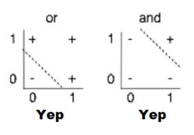
AND OR 문제는 선형적으로 구분이 가능하다. (hyperlane?)
XOR
0 + 0 = 0
1 + 1 = 0
1 + 0 = 1
0 + 1 = 1
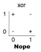
하지만 XOR 문제는 매우 단순하지만 선형적으로 구분할 수 없다.
그래서 이를 해결하기 위해 인간의 뉴런을 모방한 퍼셉트론을 층층이 쌓는 구조(Multilayer perceptrons, multilayer neural nets)가 제시 됐다.
이 신경망 층을 학습시킬 방법으로 역전파(Backpropagation) 알고리즘이 제시됐으며, 또 한가지 입력을 엄청나게 많은 단계로 나눠 분석하는 Convolutional Neural Networks(합성곱 신경망)모델 또한 제시됐다.
하지만 역전파 알고리즘의 효과가 현실의 문제를 다루기 위해 계층의 수를 늘려갈수록 희미해지는 문제가 생겼다.
그와 동시에 SVM(Support Vector Machine), 의사결정나무와 Random Forest 등의 학습 알고리즘들이 신경망의 대체제로 대두됐다.
이후 2000년대에 들어 심층신경망에서도 weight의 초기값을 잘 설정하면 학습할 수 있다는 것이 발견되었다. 이 심층 기계 학습이 기존의 모델보다 복잡한 문제를 푸는 데에 효율적이라는 것이 확인되었으며, 심층신경망(Deep neural network)을 대신해 Deep Learning(심층학습)라는 단어가 생겨났다.
이후 합성곱 신경망(Convolutional Neural Network)이 이미지 인식 분야에서 활발히 사용되었으며 이들 모델의 정확도가 기하급수적으로 상승했다.
신경망 알고리즘이 이토록 발전한 데에는 4가지의 이유가 있었다고 Geoffrey Hinton이 제시했다.
- 과거의 데이터셋이 현재보다 수 천배는 작았다.
- 컴퓨터의 성능이 예전보다 수 천, 수 백만 배 발달했다.
- weight를 제대로 초기화할 수 있게 됐다.
- 비선형성의 잘못된 유형을 사용했다.
신경망으로 XOR 문제 풀기
세 개의 weight 행렬과 3개의 bias값, 3개의 출력 – 퍼셉트론에 각각 sigmoid 함수를 취하면 XOR 문제를 풀 수 있다.
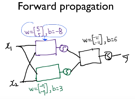
이를 하나의 신경망이라고 볼 수 있다.
또 XOR 문제를 풀 때 두 개의 퍼셉트론이 앞에서 마지막 퍼셉트론의 입력이 되었는데 이 두 개의 퍼셉트론의 weight 값과 bias 값을 행렬로 묶어 사용할 수 있다.
출력 : \(K(x) = sigmoid(XW_1+b_1)\)
K(X)를 입력으로 받아 값 예측 : \(Y=H(X) = sigmoid(K(X)W_2+b_2)\)
K = tf.sigmoid(tf.matmul(X, W_1)+b1)
hypothesis = tf.sigmoid(tf.matmul(K,W_2)+b2)
Write in code
먼저 신경망을 사용하기에 앞서 Logistic Regression을 사용해보자.
import tensorflow as tf
import numpy as np

xy = np.loadtxt('train.txt', unpack=True)
x_data = xy[0:-1]
y_data = xy[-1]

X = tf.placeholder(tf.float32)
Y = tf.placeholder(tf.float32)

W = tf.Variable(tf.random_uniform([1, len(x_data)], -1.0, 1.0))

# Our hypothesis
h = tf.matmul(W, X)
hypothesis = tf.div(1., 1.+tf.exp(-h))

# Cross entropy cost function
cost = -tf.reduce_mean(Y*tf.log(hypothesis) + (1-Y)*tf.log(1-hypothesis))

learning_rate = tf.Variable(0.01)
optimizer = tf.train.GradientDescentOptimizer(learning_rate)
train = optimizer.minimize(cost)

init = tf.global_variables_initializer()


with tf.Session() as sess:
    sess.run(init)

    for step in range(5001):
        sess.run(train, feed_dict={X:x_data, Y:y_data })
        if step % 500 == 0:
            print(step, sess.run(cost, feed_dict={X:x_data, Y:y_data}), sess.run(W))

    # Test model
    correct_prediction = tf.equal(tf.floor(hypothesis+0.5), Y)
    # Calculate Accuracy
    accuracy = tf.reduce_mean(tf.cast(correct_prediction, "float"))
    print(sess.run([hypothesis, tf.floor(hypothesis+0.5), correct_prediction, accuracy],
                    feed_dict={X:x_data, Y:y_data}))
    print("Accuracy:", accuracy.eval({X:x_data, Y:y_data}))

>>

0 0.802505 [[-0.650608   -0.92386967]]
1000 0.696653 [[-0.05479828 -0.20491447]]
2000 0.693323 [[ 0.02027203 -0.06013237]]
3000 0.693178 [[ 0.01846425 -0.02456744]]
4000 0.693156 [[ 0.01104733 -0.01198169]]
5000 0.69315 [[ 0.00609059 -0.0062336 ]]
[array([[ 0.5       ,  0.49844155,  0.50152266,  0.49996424]], dtype=float32), array([[ 1.,  0.,  1.,  0.]], dtype=float32), array([[False, False,  True,  True]], dtype=bool), 0.5]
Accuracy: 0.5
뭔가 이상하다!
로지스틱 회귀의 선형적인 모델로는 XOR 문제를 절대 풀 수 없다는 것을 알게 되었다.
그렇다면 신경망으로 문제를 풀면 어떻게 될까?
import tensorflow as tf
import numpy as np

xy = np.loadtxt('train.txt', unpack=True)
x_data = np.transpose(xy[0:-1])
y_data = np.reshape(xy[-1],(4,1))

X = tf.placeholder(tf.float32)
Y = tf.placeholder(tf.float32)

# define 2 layer Neural Network
W1 = tf.Variable(tf.random_uniform([2, 2], -1.0, 1.0))
W2 = tf.Variable(tf.random_uniform([2, 1], -1.0, 1.0))

b1 = tf.Variable(tf.zeros([2]), name="Bias1")
b2 = tf.Variable(tf.zeros([1]), name="Bias2")

# Our hypothesis
L2 = tf.sigmoid(tf.matmul(X, W1)+b1)
hypothesis = tf.sigmoid(tf.matmul(L2, W2)+b2)

# Cross entropy cost function
cost = -tf.reduce_mean(Y*tf.log(hypothesis) + (1-Y)*tf.log(1-hypothesis))

# For this time, learning rate is very important.
learning_rate = tf.Variable(0.1)
optimizer = tf.train.GradientDescentOptimizer(learning_rate)
train = optimizer.minimize(cost)

init = tf.global_variables_initializer()


with tf.Session() as sess:
    sess.run(init)

    for step in range(7001):
        sess.run(train, feed_dict={X:x_data, Y:y_data})
        if step % 500 == 0:
            print(step, sess.run(cost, feed_dict={X:x_data, Y:y_data}))

    # Test model
    correct = tf.equal(tf.floor(hypothesis+0.5), Y)
    # Calculate Accuracy
    accuracy = tf.reduce_mean(tf.cast(correct, "float"))
    print(sess.run([hypothesis],feed_dict={X:x_data, Y:y_data}))
    print("Accuracy:", accuracy.eval({X:x_data, Y:y_data}))

>>

0 0.752529
500 0.690919
1000 0.686872
1500 0.673819
2000 0.637046
2500 0.581493
3000 0.529076
3500 0.419784
4000 0.222037
4500 0.122611
5000 0.0805631
5500 0.0590243
6000 0.0462274
6500 0.0378348
7000 0.0319403
[array([[ 0.03706356],
       [ 0.97369903],
       [ 0.9692477 ],
       [ 0.03159527]], dtype=float32)]
Accuracy: 1.0
Wide Neural Network with 2 layers
Layer의 폭을 넓게 만들어보자.
import tensorflow as tf
import numpy as np

xy = np.loadtxt('train.txt', unpack=True)
x_data = np.transpose(xy[0:-1])
y_data = np.reshape(xy[-1],(4,1))

X = tf.placeholder(tf.float32)
Y = tf.placeholder(tf.float32)

# define 2 layer Neural Network - we will use 10 units
W1 = tf.Variable(tf.random_uniform([2, 10], -1.0, 1.0))
W2 = tf.Variable(tf.random_uniform([10, 1], -1.0, 1.0))

b1 = tf.Variable(tf.zeros([10]), name="Bias1")
b2 = tf.Variable(tf.zeros([1]), name="Bias2")

# Our hypothesis
L2 = tf.sigmoid(tf.matmul(X, W1)+b1)
hypothesis = tf.sigmoid(tf.matmul(L2, W2)+b2)

# Cross entropy cost function
cost = -tf.reduce_mean(Y*tf.log(hypothesis) + (1-Y)*tf.log(1-hypothesis))

# For this time, learning rate is very important.
learning_rate = tf.Variable(0.1)
optimizer = tf.train.GradientDescentOptimizer(learning_rate)
train = optimizer.minimize(cost)

init = tf.global_variables_initializer()


with tf.Session() as sess:
    sess.run(init)

    for step in range(30001):
        sess.run(train, feed_dict={X:x_data, Y:y_data})
        if step % 2000 == 0:
            print(step, sess.run(cost, feed_dict={X:x_data, Y:y_data}))

    # Test model
    correct = tf.equal(tf.floor(hypothesis+0.5), Y)
    # Calculate Accuracy
    accuracy = tf.reduce_mean(tf.cast(correct, "float"))
    print(sess.run([hypothesis],feed_dict={X:x_data, Y:y_data}))
    print("Accuracy:", accuracy.eval({X:x_data, Y:y_data}))

>>

0 0.703788
2000 0.604309
4000 0.116693
6000 0.0321776
8000 0.016299
10000 0.0104688
12000 0.00756811
14000 0.00586587
16000 0.0047586
18000 0.00398611
20000 0.0034191
22000 0.00298666
24000 0.00264682
26000 0.00237325
28000 0.00214859
30000 0.00196104
[array([[ 0.00138587],
       [ 0.99789822],
       [ 0.99809533],
       [ 0.00244387]], dtype=float32)]
Accuracy: 1.0
넓은 네트워크의 장점?
기본 크기의 네트워크에서는 learning rate 0.1 기준 7000 epoch에서야 Accuracy 1.0에 도달했지만 넓은 신경망에서는 2000번 안에 Accuracy 1.0에 도달했다.
Deep Neural Network for XOR
이번엔 레이어의 숫자를 늘려 깊은 네트워크를 만들어보자.
import tensorflow as tf
import numpy as np

xy = np.loadtxt('train.txt', unpack=True)
x_data = np.transpose(xy[0:-1])
y_data = np.reshape(xy[-1],(4,1))

X = tf.placeholder(tf.float32)
Y = tf.placeholder(tf.float32)

# define 2 layer Neural Network - we will use 3 layers.
W1 = tf.Variable(tf.random_uniform([2,10], -1.0, 1.0))
W2 = tf.Variable(tf.random_uniform([10,5], -1.0, 1.0))
W3 = tf.Variable(tf.random_uniform([5,1], -1.0, 1.0))

b1 = tf.Variable(tf.zeros([10]), name="Bias1")
b2 = tf.Variable(tf.zeros([5]), name="Bias2")
b3 = tf.Variable(tf.zeros([1]), name="Bias3")

# Our hypothesis
L2 = tf.sigmoid(tf.matmul(X, W1) + b1)
L3 = tf.sigmoid(tf.matmul(L2, W2) + b2)
hypothesis = tf.sigmoid(tf.matmul(L3, W3) + b3)

# Cross entropy cost function
cost = -tf.reduce_mean(Y*tf.log(hypothesis) + (1-Y)*tf.log(1-hypothesis))

# For this time, learning rate is very important.
learning_rate = tf.Variable(0.1)
optimizer = tf.train.GradientDescentOptimizer(learning_rate)
train = optimizer.minimize(cost)

init = tf.global_variables_initializer()


with tf.Session() as sess:
    sess.run(init)

    for step in range(30001):
        sess.run(train, feed_dict={X:x_data, Y:y_data})
        if step % 2000 == 0:
            print(step,
                  sess.run(cost, feed_dict={X:x_data, Y:y_data})
                  #sess.run(W1),
                  #sess.run(W2)
                 )

    # Test model
    correct = tf.equal(tf.floor(hypothesis+0.5), Y)
    accuracy = tf.reduce_mean(tf.cast(correct, "float"))

    print(sess.run([hypothesis],feed_dict={X:x_data, Y:y_data}))
    print("Accuracy:", accuracy.eval({X:x_data, Y:y_data}))

>>

0 0.80091
2000 0.689344
4000 0.570757
6000 0.0245225
8000 0.00782288
10000 0.00440981
12000 0.00301607
14000 0.00227221
16000 0.00181371
18000 0.00150441
20000 0.00128241
22000 0.00111577
24000 0.000986241
26000 0.000882844
28000 0.000798443
30000 0.000728336
[array([[  4.67570469e-04],
       [  9.99323130e-01],
       [  9.99140620e-01],
       [  9.08377231e-04]], dtype=float32)]
Accuracy: 1.0
Deep 하면?
epoch를 적게(2000) 주었을 때에는 2 Layer Wide NN보다 못한 성과를 내었으나 step을 많이 반복하자 더 효율적이라는 걸 깨달았다.
고려해볼 점
- Learning rate(학습률)
- Epoch(step)
- 레이어의 개수
실험
import tensorflow as tf
import numpy as np

xy = np.loadtxt('train.txt', unpack=True)
x_data = np.transpose(xy[0:-1])
y_data = np.reshape(xy[-1],(4,1))

X = tf.placeholder(tf.float32)
Y = tf.placeholder(tf.float32)

# define 2 layer Neural Network - we will use 3 layers.
W1 = tf.Variable(tf.random_uniform([2,10], -1.0, 1.0))
W2 = tf.Variable(tf.random_uniform([10,10], -1.0, 1.0))
W3 = tf.Variable(tf.random_uniform([10,10], -1.0, 1.0))
W4 = tf.Variable(tf.random_uniform([10,1], -1.0, 1.0))

b1 = tf.Variable(tf.zeros([10]), name="Bias1")
b2 = tf.Variable(tf.zeros([10]), name="Bias2")
b3 = tf.Variable(tf.zeros([10]), name="Bias3")
b4 = tf.Variable(tf.zeros([1]), name="Bias4")

# Our hypothesis
L2 = tf.sigmoid(tf.matmul(X, W1) + b1)
L3 = tf.sigmoid(tf.matmul(L2, W2) + b2)
L4 = tf.sigmoid(tf.matmul(L3, W3) + b2)
hypothesis = tf.sigmoid(tf.matmul(L4, W4) + b4)

# Cross entropy cost function
cost = -tf.reduce_mean(Y*tf.log(hypothesis) + (1-Y)*tf.log(1-hypothesis))

# For this time, learning rate is very important.
learning_rate = tf.Variable(0.3)
optimizer = tf.train.GradientDescentOptimizer(learning_rate)
train = optimizer.minimize(cost)

init = tf.global_variables_initializer()


with tf.Session() as sess:
    sess.run(init)

    for step in range(30001):
        sess.run(train, feed_dict={X:x_data, Y:y_data})
        if step % 2000 == 0:
            print(step,
                  sess.run(cost, feed_dict={X:x_data, Y:y_data})
                  #sess.run(W1),
                  #sess.run(W2)
                 )

    # Test model
    correct = tf.equal(tf.floor(hypothesis+0.5), Y)
    accuracy = tf.reduce_mean(tf.cast(correct, "float"))

    print(sess.run([hypothesis],feed_dict={X:x_data, Y:y_data}))
    print("Accuracy:", accuracy.eval({X:x_data, Y:y_data}))

>>

0 0.696796
2000 0.686248
4000 0.00259796
6000 0.000818337
8000 0.00046907
10000 0.000324707
12000 0.000246691
14000 0.000198132
16000 0.000165134
18000 0.000141363
20000 0.00012339
22000 0.000109336
24000 9.80994e-05
26000 8.89045e-05
28000 8.12297e-05
30000 7.47621e-05
[array([[  5.11028848e-05],
       [  9.99920249e-01],
       [  9.99932170e-01],
       [  1.00352103e-04]], dtype=float32)]
Accuracy: 1.0