다항변수의 분류

Multinomial classification

\[[x_1 x_2 x_3] \begin{bmatrix} w_{1} \\ w_{2} \\ w_{3} \end{bmatrix} = [w_1x_1+w_2x_2+w_3x_3]\] \[[x_1 x_2 x_3] \begin{bmatrix} w_{1} \\ w_{2} \\ w_{3} \end{bmatrix} = [w_1x_1+w_2x_2+w_3x_3]\] \[[x_1 x_2 x_3] \begin{bmatrix} w_{1} \\ w_{2} \\ w_{3} \end{bmatrix} = [w_1x_1+w_2x_2+w_3x_3]\]

3번을 다 따로 계산하는 것은 번거롭다.
벡터의 곱 내적(Dot product)을 구하는 방법을 사용하자!

\[\begin{bmatrix} w_{A1} && w_{A2} && w_{A3} \\ w_{B1} && w_{B2} && w_{B3} \\ w_{C1} && w_{C2} && w_{C3} \end{bmatrix} \begin{bmatrix} x_1 \\ x_2 \\ x_3 \end{bmatrix} = \begin{bmatrix} w_{A1}x_1 + w_{A2}x_2 + w_{A3}x_3 \\ w_{B1}x_1 + w_{B2}x_2 + w_{B3}x_3 \\ w_{C1}x_1 + w_{C2}x_2 + w_{C3}x_3 \end{bmatrix} = \begin{bmatrix} \hat{y_A} \\ \hat{y_B} \\ \hat{y_C} \end{bmatrix}\]

또 Logistic Regression에서 사용했던 것처럼 우리는 classify를 하고 싶기 때문에 \(\hat{y}\)의 값이 좀 더 이산적으로 나오길 원한다. 따라서 모든 \(\hat{y}\)에 대해 하나의 함수를 적용시켜주면 좋지 않을까?

Cost function

\[\sum \log i(\hat{y_i})=\sum_iL_i\odot -\log(\hat{y_i})\]

\(-\log(\hat{y_i})\) sigmoid 함수를 이용하기 때문에 \(\hat{y}\)가 y와 같을 때 비용은 0이 되고 \(\hat{y}\)가 y와 다를 때 비용은 무한히 커지게 된다.

이와 같은 cost function을 cross entropy라고 한다.

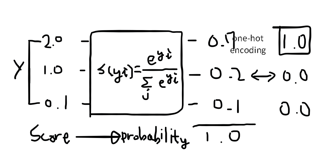
\[-\sum_i L_i log(S_i)\]

응용하면

\[C(H(x),y) = -ylog(H(x)) - (1 - y)log(1 - H(x))\] \[-\sum_i L_i log(S_i) = -\sum_i L_i log(S_i) = \sum_i L_i \odot - \log(S_i)\]

로지스틱 함수와 같은 역할을 한다고 볼 수 있다.

\[Loss = \frac{1}{N} \sum_i D(S(WX_i+b)L_i)\]

import tensorflow as tf
import numpy as np

xy = np.loadtxt('train.txt', unpack=True, dtype='float32')

x_data = np.transpose(xy[0:3])
y_data = np.transpose(xy[3:])

#Input
X = tf.placeholder("float", [None, 3])
Y = tf.placeholder("float", [None, 3])

#Weights
W = tf.Variable(tf.zeros([3,3]))

#Our model
hypothesis = tf.nn.softmax(tf.matmul(X, W))

#minimize error using cross entropy
learning_rate = 0.001

#Cross entropy
cost = tf.reduce_mean(-tf.reduce_sum(Y * tf.log(hypothesis), reduction_indices=1))

#Gradient Descent
optimizer = tf.train.GradientDescentOptimizer(learning_rate).minimize(cost)

# Initialize
init = tf.global_variables_initializer()

#Launch graph
with tf.Session() as sess:
    sess.run(init)

    for step in range(5001):
        sess.run(optimizer, feed_dict={X:x_data, Y:y_data})
        if step % 1000 == 0:
            print(step, sess.run(cost, feed_dict={X:x_data, Y:y_data}), sess.run(W))

    print("\n")

    a = sess.run(hypothesis, feed_dict={X:[[1,11,7]]})
    print(a,sess.run(tf.arg_max(a, 1)))

    b = sess.run(hypothesis, feed_dict={X:[[1,3,4]]})
    print(a,sess.run(tf.arg_max(b, 1)))

    c = sess.run(hypothesis, feed_dict={X:[[1,1,0]]})
    print(a,sess.run(tf.arg_max(c, 1)))

    all = sess.run(hypothesis, feed_dict={X:[[1,11,7],[1,3,4],[1,1,0]]})
    print(all, sess.run(tf.arg_max(all, 1)))

>>

0 1.09774 [[ -8.33333252e-05   4.16666626e-05   4.16666480e-05]
 [  1.66666694e-04   2.91666773e-04  -4.58333408e-04]
 [  1.66666636e-04   4.16666706e-04  -5.83333429e-04]]
1000 1.02354 [[-0.10928574 -0.02282181  0.13210757]
 [ 0.02266254 -0.02678034  0.00411783]
 [ 0.02685853  0.08210357 -0.10896212]]
2000 0.985988 [[-0.21581143 -0.05025396  0.26606542]
 [ 0.02894915 -0.06228962  0.03334056]
 [ 0.04230019  0.12409624 -0.16639642]]
3000 0.95411 [[-0.31725991 -0.07705297  0.39431274]
 [ 0.0336593  -0.08655652  0.05289738]
 [ 0.0584402   0.1547873  -0.21322735]]
4000 0.926335 [[-0.41402569 -0.10293558  0.51696134]
 [ 0.03758517 -0.10280674  0.06522179]
 [ 0.07442016  0.17733486 -0.25175497]]
5000 0.901696 [[-0.5065074  -0.12772508  0.63423264]
 [ 0.04120506 -0.1133228   0.07211792]
 [ 0.08978193  0.19396654 -0.2837483 ]]


[[ 0.53329509  0.2951085   0.17159635]] [0]
[[ 0.53329509  0.2951085   0.17159635]] [1]
[[ 0.53329509  0.2951085   0.17159635]] [2]
[[ 0.53329509  0.2951085   0.17159635]
 [ 0.31603345  0.44044486  0.24352166]
 [ 0.18252464  0.22840941  0.58906591]] [0 1 2]