Tensorflow 설치하기
pip install tensorflow
Hello, Tensor
import tensorflow as tf

# Node
hello = tf.constant('Hello, Tensor!')

# Start tf session
sess = tf.Session()

print(hello) # Hello is operation, tensor.
sess.run(hello)

Tensor("Const:0", shape=(), dtype=string)
Out[1]: b'Hello, World!'
변수다루기
a = tf.constant(2)
b = tf.constant(3)

c = a+b

sess.run(c)
Out[2]: 5
Placeholder 사용하기
# 변수의 type만 정해준다.
c = tf.placeholder(tf.int16)
d = tf.placeholder(tf.int16)

# everything is operation
add = tf.add(c,d)
mul = tf.mul(c,d)

# 세션 실행 및 placeholder 값 지정
with tf.Session() as sess:
    print ("Addition with variables: %i" % sess.run(add, feed_dict={c:2, d:3}))
    print ("Multiplication with variables: %i" % sess.run(mul, feed_dict={c:2, d:3}))

>>Addition with variables: 5
>>Multiplication with variables: 6
Hypothesis and Cost
\[H(x) = Wx + b\] \[cost(W, b) = \frac{1}{m} \sum_{i=1}^{m} (H(x^{(i)}) - y^{(i)})^2\]Simplified cost function
\[H(x) = Wx\] \[cost(W) = \frac{1}{m} \sum_{i=1}^{m} (Wx^{(i)} - y^{(i)})^2\]H(x)가 y값에 근접할 수록 cost 값은 줄어들게 된다.
cost 값을 줄이기 위해 사용하는 것이 경사하강법(Gradient descent)이다.
Gradient Descent
- (0,0)이나 아무 지점에서 시작해도 괜찮다.
- W와 b값을 조금씩 바꿔가며 cost를 줄이기 위해 시도한다.
- 주어진 그래프에서 경사를 구하기 위해 미분을 한다.
Convex function
-
사실 cost function의 모양이 복잡해지면 복잡해질수록 Gradient Descent의 시작점에 따른 도달점이 달라지게 된다. 이 때 어느점에서 시작하던 가장 낮은 cost에 도달할 수 있는 함수를 convex function이라고 부른다. 따라서 cost function을 설계할 때 이것의 모양이 convex function을 이루는지 확인해야 한다.
-
하지만 현실의 문제를 다룰 경우 cost function이 수십~ 그 이상의 차원을 가져 복잡한 구조를 이루고 있기 때문에 convex function을 찾을 수 없을 가능성이 높다.
Linear Regression
# 데이터
x_data = [1,2,3]
y_data = [4,5,6]

# 무작위 수
W = tf.Variable(tf.random_uniform([1], -1.0, 1.0))
b = tf.Variable(tf.random_uniform([1], -1.0, 1.0))

# Placeholder
X = tf.placeholder(tf.float32)
Y = tf.placeholder(tf.float32)

# 가설
hypothesis = W * X + b # Y = 1x+3

# cost function
cost = tf.reduce_mean(tf.square(hypothesis - Y))

# Train by gradient descent
a = tf.Variable(0.1) # learning rate, alpha
optimizer = tf.train.GradientDescentOptimizer(a)
train = optimizer.minimize(cost)

# Initialize variables
init = tf.global_variables_initializer()

sess = tf.Session()
sess.run(init)

"""
Placeholder를 사용하면 Session을 시작할 때 값을 정해주어
모델을 쉽게 재활용할 수 있다.
"""

for step in range(2001):
    sess.run(train, feed_dict={X:x_data, Y:y_data})
    if step % 50 == 0 : # epoch 50마다 결과 출력
        print(step, sess.run(cost, feed_dict={X:x_data, Y:y_data}), sess.run(W), sess.run(b))

# train된 hypothesis를 이용해 예측
print(sess.run(hypothesis, feed_dict={X:5}))
print(sess.run(hypothesis, feed_dict={X:2.5}))

>>

0 0.919434 [ 2.13872838] [ 0.9569912]
50 0.0571887 [ 1.27774811] [ 2.36861348]
100 0.00501811 [ 1.08227479] [ 2.81297016]
150 0.000440327 [ 1.0243715] [ 2.94459796]
200 3.86367e-05 [ 1.00721931] [ 2.98358893]
250 3.39094e-06 [ 1.00213861] [ 2.99513841]
300 2.97692e-07 [ 1.0006336] [ 2.99855971]
350 2.61831e-08 [ 1.00018775] [ 2.99957299]
400 2.29503e-09 [ 1.00005567] [ 2.9998734]
450 2.0079e-10 [ 1.00001645] [ 2.99996281]
500 1.83415e-11 [ 1.00000489] [ 2.99998879]
550 1.91373e-12 [ 1.00000167] [ 2.99999619]
600 1.91373e-12 [ 1.00000167] [ 2.99999619]
650 1.91373e-12 [ 1.00000167] [ 2.99999619]
700 1.91373e-12 [ 1.00000167] [ 2.99999619]
750 1.91373e-12 [ 1.00000167] [ 2.99999619]
800 1.91373e-12 [ 1.00000167] [ 2.99999619]
850 1.91373e-12 [ 1.00000167] [ 2.99999619]
900 1.91373e-12 [ 1.00000167] [ 2.99999619]
950 1.91373e-12 [ 1.00000167] [ 2.99999619]
...
2000 1.91373e-12 [ 1.00000167] [ 2.99999619]
[ 8.00000477] # 잘 작동한다. (y = 1x + 3)
[ 5.50000048]
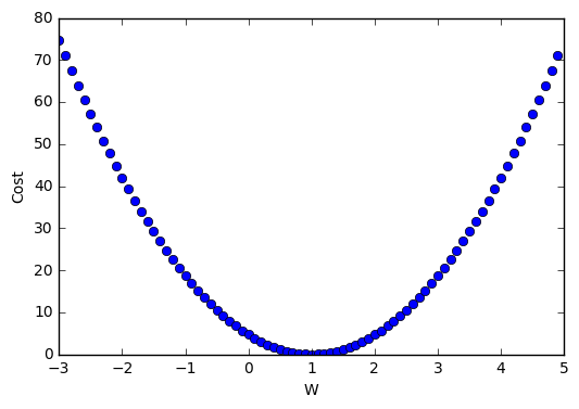
Minimizing Cost
X = [1., 2., 3.]
Y = [1., 2., 3.]
m = n_samples = len(X)

# Set model weight
W = tf.placeholder(tf.float32)

# Linear model
hypothesis = tf.mul(X, W)

# Cost function
cost = tf.reduce_sum(tf.pow(hypothesis-Y, 2))/(m)

# Initialize
init = tf.global_variables_initializer()

# For graphs
W_val = []
cost_val = []

# Launch the graph
sess = tf.Session()
sess.run(init)
for i in range(-30, 50):
    print(i*0.1, sess.run(cost, feed_dict={W: i*0.1}))
    W_val.append(i*0.1)
    cost_val.append(sess.run(cost, feed_dict={W: i*0.1}))

# Graphic display
plt.plot(W_val, cost_val, 'bo')
plt.ylabel('Cost')
plt.xlabel('W')
plt.show()
cost = tf.reduce_sum(tf.pow(hypothesis-Y, 2))/(m)
\(cost(W) = \frac{1}{m} \sum^m_{i=1}(Wx^{(i)}-y^{(i)})^2\)
X = [1., 2., 3.]
Y = [4., 5., 6.]
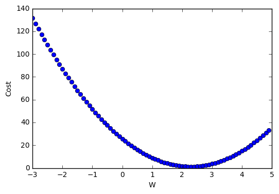
descent = W - tf.mul(0.1, tf.reduce_mean(tf.mul((tf.mul(W, X) - Y), X)))
\(W := W - \alpha \frac{1}{m} \sum^m_{i=1}(Wx^{(i)}-y^{(i)})x^{(i)}\)
\(\alpha\)는 graph에서 어느정도 내려가야 할지를 나타내는 변수이며, \((W_x^{(i)}-y^{(i)})x^{(i)}\)부분이 기울기를 나타낸다. 기울기가 -일 경우 w를 +로 이동시키고, 기울키가 +일 경우에는 w를 -로 이동시켜 최종적으로 원하는 값을 찾을 수 있다.
x_data = [1., 2., 3.,]
y_data = [1., 2., 3.,]

W = tf.Variable(tf.random_uniform([1], -10.0, 10.0))

X = tf.placeholder(tf.float32)
Y = tf.placeholder(tf.float32)

hypothesis = W * X

cost = tf.reduce_mean(tf.square(hypothesis - Y))

descent = W - tf.mul(0.1, tf.reduce_mean(tf.mul((tf.mul(W, X) - Y), X)))
update = W.assign(descent)

# initialize

init = tf.global_variables_initializer()

sess = tf.Session()
sess.run(init)

for step in range(30):
    sess.run(update, feed_dict={X:x_data, Y:y_data})
    print(step, sess.run(cost,  feed_dict={X:x_data, Y:y_data}), sess.run(W))

>>

0 27.4124 [-1.42364931]
1 7.79729 [-0.29261291]
2 2.2179 [ 0.31060648]
3 0.630868 [ 0.6323235]
4 0.179447 [ 0.80390584]
5 0.0510427 [ 0.89541644]
6 0.0145188 [ 0.94422209]
7 0.00412979 [ 0.9702518]
8 0.00117469 [ 0.98413432]
9 0.000334136 [ 0.99153829]
10 9.50439e-05 [ 0.99548709]
11 2.7035e-05 [ 0.9975931]
12 7.68948e-06 [ 0.99871635]
13 2.18712e-06 [ 0.99931538]
14 6.221e-07 [ 0.99963486]
15 1.76933e-07 [ 0.99980527]
16 5.02863e-08 [ 0.99989617]
17 1.43152e-08 [ 0.99994463]
18 4.05883e-09 [ 0.9999705]
19 1.15551e-09 [ 0.99998426]
20 3.30617e-10 [ 0.9999916]
21 9.2727e-11 [ 0.99999553]
22 2.65269e-11 [ 0.99999762]
23 7.46188e-12 [ 0.99999875]
24 1.92912e-12 [ 0.99999934]
25 5.16328e-13 [ 0.99999964]
26 1.29082e-13 [ 0.99999982]
27 9.9476e-14 [ 0.99999988]
28 2.4869e-14 [ 0.99999994]
29 0.0 [ 1.]